Finding out how to reduce the GPU frame time for rendering applications on a personal computer can be a challenging task, even for the most experienced PC game developers. This blog post describes our performance categorization method used internally at NVIDIA to use NVIDIA-specific hardware metrics to find the main performance limiter for any given GPU workload (also known as a performance tag or call scope).
Our performance classification approach does not begin with assumptions or knowledge about the content presented on the GPU. Instead, it only starts with hardware metrics, letting us know the utilization of the entire GPU, which hardware units and subunits limit performance, and how close they are to their respective peak performance (also known as "speed light" or "SOL". ). If your application does not use asynchronous computations , you can map this hardware-centric information back to what the graphics API and shaders are doing, providing guidance on how to improve GPU performance for any given workload:
If there is no GPU unit with high throughput (compared to SOL), we will strive to increase the throughput of at least one unit.
If some GPU units have a higher throughput (compared to SOL) then we will figure out how to remove the work from this unit.
 Nsight Range Profiler
Starting with Kepler Architecture 1 ( full support for Maxwell , Pascal, and Volta GPUs) , the PerfWorks library on DX11, DX12, and OpenGL on all NVIDIA GPUs can capture hardware metrics for each GPU workload . Although PerfWorks header files have not been made public, the library is now available through common tools: Nsight 's Range Profiler : Visual Studio Edition 5.5 for DX12, DX11 and OpenGL 4.6 (but not Vulkan), and Microsoft's " PIX on Windows " For DX12.
1 From Wikipedia you can see that the GeForce 600 and 700 series are mostly Kepler, the 900 series is Maxwell, the 1000 series is Pascal, and TITAN V is Volta.
Step 1: Lock the GPU core clockFirst of all, in order to get the most definitive measurement results, we recommend that you always lock your GPU core clock frequency before collecting any performance metrics (and unlock after unlocking for optimal performance, and if the GPU is idle or just minimal Desktop Rendering for Power Consumption and Noise). On Windows 10 with "developer mode" enabled, this can be done by running a simple DX12 application that calls SetStablePowerState (TRUE) on a virtual DX12 device and then enters without releasing the device. the sleep state, as the blog.
Note: Starting with Nsight: Visual Studio version 5.5, Range Profiler can now effectively call SetStablePowerState() before/after any Range analysis, using the internal driver API for all Windows versions (not just Windows 10), nor The operating system is required to be in "developer mode". Therefore, when using the Nsight Range Profiler, you do not have to worry about locking the GPU Core clock.
Step 2: Capture the picture with Nsight HUDFor non-UWP (universal Windows platform) applications, this can be done by dragging and dropping your EXE (or batch file) to Nsight 's " NVIDIA Nsight HUD Launcher " shortcut installed on the desktop to achieve what you want The location of the game is captured then:
Press CTRL-Z to display Nsight HUD in the upper right part of the screen, and
Click on the Pause and Capture Frame button in the Nsight HUD , or press the space bar to start capturing.
You can export the current frame to a Visual Studio C++ project by clicking the " Save capture to disk " button . (By default, Nsight exported frames are saved to C:\Users\Documents\NVIDIA Nsight\Captures...)
You can click " Resume " to continue playing your game to find other places where you want to capture more frames.
Note: You can skip the " Save Capture to Disk " step and skip directly to the next step (Scrubber & Range Profiler Analysis), but we recommend always saving the captures to disk and archiving them so that you can return to them later you need to . Saving the exported frames to disk allows you to later attach the data to the analysis so that you or others in the team can try to reproduce your results.
In NVIDIA, we consider performance analysis as a scientific process, we provide all repro data related to analysis, and encourage colleagues to re-draw and review our results. In our experience, it is also a good practice to capture frames before and after performance optimization attempts, whether successful or not, to analyze how hardware metrics change and learn from the results.
Additional instructions for Nsight frame capture:
For the Nsight framework, it doesn't matter whether your application is running in windowed, full-screen, or full-screen, borderless mode, because Nsight always runs the framework in a hidden window. Just make sure the resolution and graphics settings are what you want to analyze.
For DX12 applications, we assume that asynchronous calculations are not used, otherwise some hardware metrics may be affected by multiple simultaneous execution workloads on the GPU. So far, for all PerfWorks-based analyses, we recommend disabling asynchronous computing in DX12 applications.
Regarding DX12 asynchronous replication calls (in the COPY queue), these calls can be used in frame captures, but you should be aware that PerfWorks and Nsight currently do not analyze COPY queue calls separately. Therefore, any COPY queue call executed in parallel with other DIRECT queue calls can affect GPU DRAM traffic in these workloads.
Dragging and dropping the exe file to the Nsight HUD Launcher will not apply to UWP applications. In the practice of the UWP Nsight launched, currently only supports the Visual Studio IDE through.
Step 3: Decompose GPU frame timeA top-down view of GPU time is a good way to find out which performance indicators/workloads are the most expensive in a frame. For the HBAO + DX11 test application, the SSAO is rendered at 4K on the GeForce GTX 1060 6GB. In Nsight Scrubber, the GPU frame time decomposition is as follows:
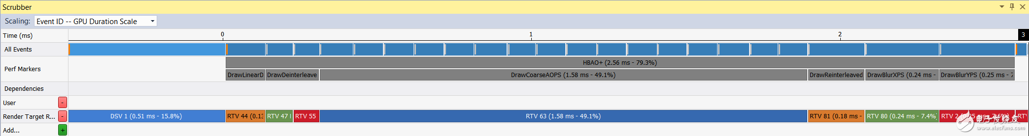 Figure 1. Sample GPU frame-time breakdown of Scrubber in Nsight: Visual Studio Edition 5.5.
In the Perf Markers row, Scrubber shows the GPU time for each workload measured by the D3D timestamp query, and the percentage of GPU frame time that each workload is using (excluding the current call). In the example of Figure 1, it is obvious which workload is the most expensive in this frame: "DrawCoarseAOPS", accounting for 49.1% of the GPU time.
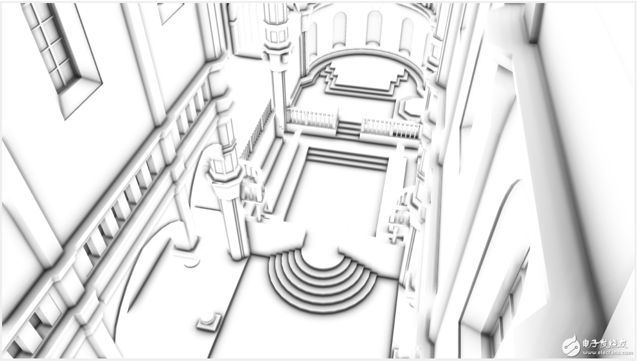
Note: To redisplay this result, download the HBAO + source code version 3.1 from GitHub and run the "SampleApp_D3D11" project in Visual Studio. To make a RenderAO call to issue performance flags, you can define ENABLE_PERF_MARKERS = 1 in the GFSDK_SSAO_D3D11 -> Project Properties -> C/C + -> Preprocessor. For the record, here is what the frame looks like:
 Step 4: Start Nsight Range Profiler
 You can open the frame capture Visual Studio solution file you exported to disk in step 2, build the solution in Release x64, then go to the Nsight menu in Visual Studio and click Start Graphics Debug .
To reach Nsight Range Profiler, you can start Nsight Frame Capture EXE and then:
Press CTRL-Z and then press the space bar
ALT-Tab to Your Visual Studio Window
Find Scrubber Tabs Added by Nsight
Right-click on the workload you want to analyze and click " Profile [Perf Markers] ... "
Note: If for some reason CTRL-Z + SPACE does not apply to your application, you can ALT-Tab to Visual Studio, and then click Visual Studio -> Nsight Menu -> Pause and Capture Frames.
We call Range Profiler from the “DrawCoarseAOPS†workload in step 3 by right-clicking on the “DrawCoarseAOPS†box in the scrubber and executing “Profile [Perf Markers] DrawCoarseAOPS†(only by analyzing this call scope, but otherwise other)
 Figure 2. Starting Nsight Range Profiler for a given workload from the Scrubber window.
Range Profiler injects PerfWorks calls in Nsight frame captures and collects a set of PerfWorks metrics for the specified workload. After the analysis is complete, Nsight will display the collected metrics in a new section of the Range Profiler window under Scrubber.
Step 5: Check Top SOL and Cache Hit RateWe first check the "Pipeline Overview" Summary section of the Range Profiler. This is just a view of PerfWorks's measurement of current workloads. By hovering over any metric, the actual Perfworks metric name will be displayed in the tooltip:
 Figure 3. Nsight Range Profiler tooltip showing the PerfWorks metric name and description.
The primary top metric to look at for each workload is the SOL% per unit metric for the GPU. These communicate the proximity of each unit to its maximum theoretical throughput or speed of light (SOL). At a high level, per-cell SOL% metrics can be thought of as the ratio of achieved throughput to SOL throughput. However, for cells with multiple subunits or concurrent data paths, SOL% per cell is the maximum of all sub-SOL standards for all subunits and data paths.
Note: If you are unfamiliar with the names of devices in the GPU, read the following blog post that provides a high-level overview of how the logical graphics pipeline maps to GPU cells in the GPU architecture: " The life of the triangle - NVIDIA's logic pipeline, " and GTC Slides 7 through 25 in the 2016 presentation: " GPU Driven Rendering ." under these circumstances:
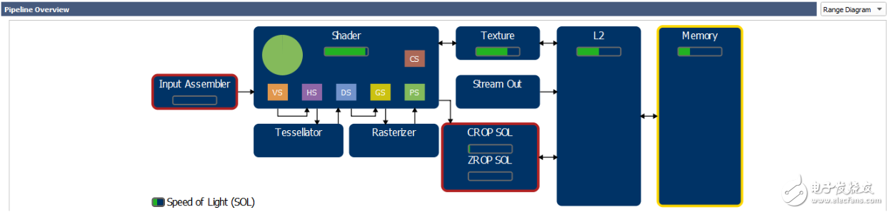
The "IA" (Input Assembler) loads the index and vertex (before the vertex shader is called).
SM (streaming multiprocessor) runtime shader.
TEX performs SRV extraction (and drone access since Maxwell ).
L2 is a secondary cache connected to each DRAM partition.
CROP color writes and blend render targets.
ZROP performs depth mask testing.
DRAM ("Memory" in the range graph) is GPU video memory.
Note: In the Nsight Range Profiler results, you can find a simplified view of the graphics pipeline and its mapping to the GPU unit by selecting Range Diagram in the pipeline overview. In the figure, the SOL% value per unit is shown as a green bar:
 Figure 4. Nsight Range Profiler: Pipeline Overview -> Range Diagram.
As shown in Figure 4, today's GPU is not a simple linear pipeline (A → B → C → ...) but an interconnected unit network (SM <-> TEX <-> L2, SM-> CROP < -> L2, etc.) Simple "bottleneck" calculations depend on the fixed upstream and downstream interfaces of each unit, but are not sufficient to infer the performance of the GPU. Therefore, in conducting our analysis, we mainly examine the SOL% metrics for each unit to determine the unit and/or limit performance issues. The next section will discuss this method in detail.
5.2. "Top SOL Units"In our performance classification methodology, we always start by looking at the first 5 SOL units and their related SOL% metrics. These are the first five hardware units that limit the GPU performance of this workload. Nsight Range Profiler displays the first 5 SOL% metrics (aka "top SOL") in the Pipeline Overview - Summary section, for example:
 Figure 5. Top SOLs example in Range Profiler -> Pipeline Overview: Visual Studio Edition 5.5 in Nsight.
If the top-level SOL% value is greater than 80%, then we know that the configuration file workload on the GPU runs very efficiently (close to the maximum throughput), in order to speed up, we should try to remove the work from the top-level SOL unit and it goes to another unit. For example, for SM workloads as top-level SOL units with SOL%> 80%, it is possible to attempt to skip instruction groups opportunistically, or consider moving certain calculations to lookup tables. Another example is moving a structured buffer load to a constant buffer load in shaders in a unified access structured buffer (all threads load data from the same address) and a workload that is limited by texture throughput ( Because the structured buffer is loaded via the TEX unit).
Case 2: Top SOL% < 60%If the highest SOL% value is <60%, this means that the top-level SOL unit and all other GPU units with lower SOL% are underutilized (idle cycles), run inefficiently (stall cycle), or their fast path is not reached, for the reason It is the details of the workload they give. Examples of these situations include:
The application is partially limited by the CPU (see Section 6.1.1);
A large number of waiting idle commands or graphics <-> computation switches repeatedly empty the GPU pipeline (see Section 6.1.2);
TEX extracts data from texture objects that have a format, dimension, or filter pattern, allowing them to run at design time with lower throughput (see these comprehensive benchmarks for GTX 1080 ). For example, when tri-linear filtering is used to sample a three-dimensional texture, 50% of TEX SOL% is expected;
Memory subsystems are inefficient, such as low cache hits in TEX or L2 units, resulting in sparse DRAM access to low DRAM SOL%, and VB/IB/CB/TEX replacing GPU DRAM from system memory;
The input component gets a 32-bit index buffer (half-rate compared to 16-bit index).
Note: In this case, we can use the highest SOL% value to derive the upper limit of the maximum gain that can be achieved on this workload by reducing inefficiency: if a given workload runs at 50% of its SOL, and Assuming that SOL% can be increased to 90% by reducing internal inefficiencies, we know that the maximum expected return on the workload is 90/50 = 1.8x = 80%.
Case 3: The highest SOL% in [60,80]In this case (gray area), we follow the scenario 1 (high SOL%) and case 2 (low SOL%) methods.
Note: The per-cell SOL% metrics are defined relative to the GPU period (wall clock), which may be different from the activity period (cycles where the hardware unit is not idle). The main reason why we define them relative to the elapsed period rather than the valid period per unit is to make the SOL% indicators comparable by giving them all the common denominators. Another benefit of defining them relative to elapsed cycles is that any GPU idle cycle that limits overall GPU performance will be reported as the lowest SOL% value for this workload (the top metric in our SOL boot classification).
5.3. Minor SOL units and TEX and L2 hit ratesThe reason that Nsight Range Profiler reports the first five SOL units is not just the largest one, as there may be multiple hardware units interacting with each other and all have limited performance to a certain extent. Therefore, we recommend manually clustering SOL units based on SOL% values. (Actually, a 10% increment seems to define these clusters well, but we recommend manually executing the cluster to avoid missing any content.)
Note: We also recommend looking at the TEX (L1) and L2 hit rates shown in the Memory section of the distance analyzer. In general, hit rates greater than 90% are good, 80% to 90% are good, and 80% or less (may significantly limit performance).
Full-screen HBAO + Fuzzy Workload with Top 5 SOLs:
SM: 94.5% | TEX: 94.5% | L2: 37.3% | Crops: 35.9% | DRAM: 27.7%...is both SM and TEX restrictions. Since the SM and TEX SOL% values ​​are the same, we can infer that the SM performance is likely to be limited by the interface throughput between the SM and TEX units: SM requests TEX or TEX to return data to the SM.
It has a TEX hit rate of 88.9% and an L2 hit rate of 87.3%.
Review the study of this workload in the "TEX-Interface Limited Workload" appendix.
Moving from the HBAO+ example, here are some typical game engine workloads that we have recently analyzed.
SSR Workload with Top Level SOL:
SM: 49.1% | L2: 36.8% | TEX: 35.8% | DRAM: 33.5% | CROP: 0.0%... Using SM as the main limiter, L2, TEX, and DRAM as secondary limiters, the TEX hit rate was 54.6%, and the L2 hit rate was 76.4%. This poor TEX hit rate can explain the low SM SOL%: Because of the poor TEX hit rate (most likely due to the neighboring pixels having very distant texels), the average TEX delay seen by SM is more than usual. High, more challenging hidden.
Note: The activity unit here is actually a dependency chain: SM -> TEX -> L2 -> DRAM.
This top SOL GBuffer fills the workload:
TEX: 54.7% | SM: 46.0% | DRAM: 37.2% | L2: 30.7% | CROP: 22.0%... Using TEX and SM as the main limiters, using DRAM and L2 as secondary limiters, the TEX hit rate was 92.5% and the L2 hit rate was 72.7%.
This tiled lighting calculation shader has top SOL:
SM: 70.4% | L2: 67.5% | TEX: 49.3% | DRAM: 42.6% | CROP: 0.0%... SM & L2 as the main limiter, TEX & DRAM as a secondary limiter, TEX hit rate was 64.3%, L2 hit rate was 85.2%.
This shadow map with top-level SOL generates the workload:
IA: 31.6%| DRAM: 19.8% | L2: 16.3% | VAF: 12.4% | CROP: 0.0%... is IA limited (input assembler) and has a low SOL%. In this case, changing the index buffer format from 32-bit to 16-bit helps. The TEX hit rate does not matter because TEX is not in the top 5 SOL units. The L2 hit rate was 62.6%.
Step 6: Learn about the performance limiterAfter completing step 5, we know the top SOL units (percentage of GPU unit names and maximum throughput) for each of the workloads of interest, as well as the TEX and L2 hit rates.
We know that the top SOL GPU units are limiting the performance of the workload being studied because these units are running the unit that is closest to its maximum throughput. We now need to understand what is limiting the performance of these top-SOL units.
6.1. If the top SOL% is lowAs described in section 5.2.2 above, there are many possible causes. We often refer to these as pathologies - and, as in real life patients, the workload may be affected by multiple conditions at the same time. We first check the values ​​of the following metrics: " GPU idle % " and " SM unit activity percentage ".
6.1.1. GPU Idle % metricThe Range Profiler 's " GPU Idle% " metric maps to the "gr__idle_pct" PerfWorks metric. It is the percentage of the elapsed GPU elapsed time for the entire graphics and compute hardware pipeline under the current workload. These "GPU idle" cycles are cycles when the CPU is unable to provide the GPU with fast enough commands so the GPU pipeline is completely empty and does not need to handle any work. Please note that pipe emptying caused by the Wait For Idle command is not counted as "GPU idle".
If you see this metric greater than 1% for any given GPU workload, you know that this workload is CPU-bound for some reason and that the performance impact of this CPU workload is at least 1%. In this case, we recommend measuring the total CPU time for each workload that the following CPU calls take, and then try to minimize the most expensive CPU time:
For DX11:
Flush {, 1}
map
UpdateSubresource {,1}
For DX12:
wait
ExecuteCommandLists
For DX11 and DX12:
Any create or release call
DX11 Description:
ID3D11DeviceContext::Flush enforces the command buffer to start, which may require the Flush() call to stop on the CPU.
When the same fragmented resource is mapped in consecutive frames, calling ID3D11DeviceContext::Map on the STAGING resource may cause the CPU to stall due to resource contention. In this case, the Map call in the current frame must wait internally until the previous frame (using the same resource) has been processed before returning.
Calling ID3D11DeviceContext::Map with DX11_MAP_WRITE_DISCARD may cause the CPU to stall due to the driver running out of version space. This is because each time a Map(WRITE_DISCARD) call is executed, the driver returns a new pointer to a fixed-size memory pool. If the driver runs out of version space, Map calls will stop.
DX12 considerations:
Each ExecuteCommandLists (ECL) call has some associated GPU idle overhead for starting a new command buffer. Therefore, in order to reduce GPU idle time, we recommend that you assign all command lists to as few ECL calls as possible unless you really want the command buffer to start at some point in the frame (for example, to reduce VR applications The input delay has a frame in flight).
When the application calls ID3D12CommandQueue:: Wait, the operating system (Windows 10) will suspend the GPU submitting a new command buffer to the command queue until the call returns.
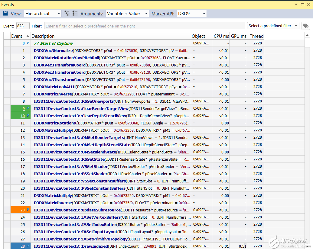
Note: The CPU time for each API call can be measured using Nsight by capturing a frame and then entering Visual Studio -> Nsight -> Windows -> Events:
The " SM unit active % " metric reports the percentage of active periods of at least 1 warp (32 threads) per SM instance, averaged across all SM instances. Please note that the transformation that is waiting for the memory request to return will be recorded as "running"/on the fly.
In Nsight:Visual Studio Edition 5.5, this metric appears in the Range Analyzer Results in the Pipeline Summary.
For full-screen quads or compute shader workloads, the SM should be active in more than 95% of the workload. If not, then there is likely to be an imbalance between SMs, some SMs are idle (no activity warping), while others are active (at least one activity warping). This happens when you run a shader with a non-uniform warping delay. In addition, serialized scheduling calls with a small number of small thread groups cannot be wide enough to fill all SMs on the GPU.
If the SM activity percentage is less than 95% for any geometry rendering workload, you know that you can achieve a performance increase on this workload by overlapping asynchronous computation work with it. On DX12 and Vulkan this can be done using the Compute-only queue. Please note that even if the percentage of SM activity is close to 100%, acceleration can be obtained from asynchronous calculations, as SM may be tracked as active but may be able to withstand more active states.
Another reason why the "percentage of SM unit activities" may be lower than 95% for any workload is the frequent GPU pipeline consumption (wait for idle command, also known as WFI), which may be due to the following reasons:
Problem: For shader scheduling reasons, many state changes when the HS and DS are active will cause the SM to disappear.
Solution: Minimize the number of state changes (including resource bindings) in the workload with refinement shaders.
Problem : Each batch of back-to-back ResourceBarrier calls on a given queue may cause all GPU work on that queue to be exhausted.
Solution : To minimize the performance impact of the ResourceBarrier call, it is important to minimize the number of locations in the frame where the ResourceBarrier call is performed.
Problem : By default, subsequent render calls with bound drones are usually conservatively separated by our driver injected GPU WFI command to prevent any data harm.
Solution : You can use the following call to disable the insertion of drone-related wait-idle commands: NvAPI_D3D11_{Begin,End} UAVOverlap or NvAPI_D3D11_BeginUAVOverlapEx.
Please note that in DX12, OpenGL and Vulkan, drone-related wait-idle commands are explicitly controlled by the application using API calls (ResourceBarrier, glMemoryBarrier, or vkCmdPipelineBarrier).
Problem : Switching between Draw and Dispatch calls in the same hardware queue can cause GPU WFI exec Wuxi Ark Technology Electronic Co.,Ltd. , https://www.arkledcn.com